OpticalSystem
| Type: | section |
|---|---|
| Appearance: | optional |
Ideally, an optical system transfers a pattern in the object plane into a perfect (de-)magnified copy in the image plane. However, this is theoretically not reachable and it becomes necessary to specify the aberrations of the optical system from the perfect imaging system. In the following the parameters and assumptions of the optical system model as used in JCMsuite are introduced step by step.
A basic assumption is that the optical system is fully specified by its transfer properties of a coherent time-harmonic electromagnetic field given by an electric field intensity  in the object plane.
In the following  denotes the wave number in the object space, where
  is the corresponding refractive index, and
  the vacuum wavenumber. On the image side,
  and
and  are defined accordingly.
The perfect system
For the moment we disregard the polarization of the electric field  and consider a scalar field
  in the object plane. An ideal optical system would produce a scaled image
  formed in the image plane:

with  ,
,  .
.  is the spot magnification and corresponds to the input parameter SpotMagnification.
Switching to the  space representation by Fourier transforming, this relation reads as

Hence, the Fourier value of the image field at  is related to the Fourier value at
  of the object field. Actually this is Abbe’s sine rule: A Fourier value
  gives rise to a plane wave
traveling in the direction of the wave vector  , where
  From a geometrical optics point of view, this wave corresponds to a light ray in the same direction. The optical system maps this ray (plane wave) to a ray with wave vector
  Regarding the propagation angles with respect to the optical axis yields

which gives Abbe’s sine rule

For the vector field  we claim that the perfect system preserves the
  , and
, and  polarization, that is

with direction vectors  ,
,  and where
  is the direction of the optical axis.
  and
and  are defined accordingly. Hence, we have

with a rotation matrix  . In the following we will skip this matrix for the sake of a simpler notation.
Numerical Aperture
Not all emitted plane waves are able to reach the image plane. For  the plane wave is evanescent and will not reach the entrance pupil. Analogously, a wave with
 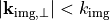 on the image side will not reach the image plane. Beside this, due the finite opening angles of the lenses, the optical system further restricts the ray bundle passing the optical system. This is is expressed either by the image side numerical aperture,

or equivalently by the object side numerical aperture

Hence, the image Fourier decomposition will only contain propagating waves fitting into the aperture:
The aberrant system
It is assumed that the one-to-one relationship between  and remains valid, but the imperfect system allows for a non-trivial coherence transfer function
  :
:

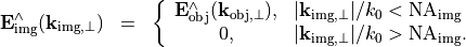
In the following, the coherence transfer function is expressed in terms of normalized pupil coordinates

and is expanded into factors according to different actions of the optical system:

The factors are in detail:
- Pupil function
 . This binary function (
 or
or  ) defines which Fourier modes are allowed to pass the optical system. The pupil function is given by the parameters NumericalAperture and InnerNumericalAperture.
 - Phase aberration
 . This scalar factor accounts for phase aberrations in the optical system due to optical path length deviations. For a detailed description see PhaseExpansion.
 - Obliquity factors
 . These scalar factor are needed to assure energy conservation. For a discussion see below in the appendix. This factor is directly incorporated by
 JCMsuiteand should not be mistaken for the energy apodization exponents .
. - Apodization exponents . These scalar factors account for apodization (damping) in the optical system due to energy losses. The object sided apodization exponent
 accounts for energy losses between the object plane and the pupil plane, whereas
  accounts for energy losses between the pupil plane and the image plane. For a detailed description see ObjectSidedApodizationExpansion or ImageSidedApodizationExpansion
 - Jones pupil functions
 . These matrix functions are used to describe polarization effects caused by the optical system. The object sided Jones matrix
  accounts for polarization effects between the object plane and the pupil plane, whereas
  accounts for polarization effects between the pupil plane and the image plane. For the precise definition see ObjectSidedJonesExpansion and ImageSidedJonesExpansion.
The Jones matrix  acts in the pupil plane as depicted in the parent section HermiteGaussianBeam. Virtually, the optical field travels through the pupil plane on rays parallel to the optical axis, so that the electric field has a vanishing
  -component. The 2-by-2 Jones matrix acts on the cartesian components of the electric field within the pupil plane:

Appendix
A) Energy considerations
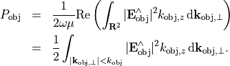
It is the aim to derive the obliquity factor 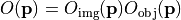 from the energy conservation principle. We adopt the notation from above. The energy flux through the object plane is given by the integral over the Poynting vector projected to the normal ()-direction:
where Parseval’s rule was used.
It follows from time-harmonic Maxwell’s equations that
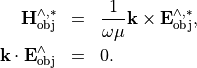
The second equality relates to the divergence condition.
Using that  , we get
The second equality holds true since  is purely imaginary for .
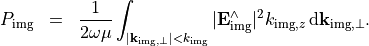
An analogue expression can be derived for the energy flux through the image plane  :
:
Disregarding inner losses, the energy contribution of the Fourier spectrum which pass the optical system, that is 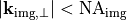 , must be equal on the object and image sides:
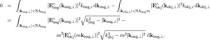
Since this should hold for any field it follows that

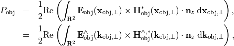
which yields a relation for the magnitudes of the image Fourier transform and the the object Fourier transform:
![\begin{eqnarray*}
|\VField{E}_{\mathrm{img}}^{\wedge}(\pvec{k}_{\mathrm{img}, \perp})| & = &
m |\VField{E}_{\mathrm{obj}}^{\wedge}(\pvec{k}_{\mathrm{obj}, \perp})|\sqrt[4]{\frac{k_{\mathrm{obj}}^2-|\pvec{k}_{\mathrm{obj}, \perp}|^2}{k_{\mathrm{img}}^2-|\pvec{k}_{\mathrm{img}, \perp}|^2}}=m |\VField{E}_{\mathrm{obj}}^{\wedge}(\pvec{k}_{\mathrm{obj}, \perp})|\sqrt{\frac{k_{z, \mathrm{obj}}}{k_{z,\mathrm{img}}}}.
\end{eqnarray*}](_images/math/2afa7845be04f3cc6e1bc4728f2371d5b58e571c.png)
In normalized coordinates this gives the obliquity factor
![\begin{eqnarray*}
O(\pvec{p}) & = & \sqrt[4]{\frac{n_\mathrm{obj}^2-|\pvec{p}|^2 \mathrm{NA}_{\mathrm{obj}}^2}{n_\mathrm{img}^2-|\pvec{p}|^2\mathrm{NA}_{\mathrm{img}}^2}}.
\end{eqnarray*}](_images/math/58d3f2d770149a4b618d8ecbceff410e81caf417.png)
For the splitting of the obliquity factor into an object-sided obliquity factor  and an image-sided obliquity factor
  we regard the pupil as an intermediate imaging with magnification equal infinity rendering each ray parallel to the optical axis, so that
  or equivalently,
  .
.
Assuming a refractive index  within the pupil plane this leads to the splitting
![\begin{eqnarray*}
O_{\mathrm{obj}}(\pvec{p}) & = & \sqrt[4]{n_\mathrm{obj}^2-|\pvec{p}|^2 \mathrm{NA}_{\mathrm{obj}}^2}, \\
O_{\mathrm{img}}(\pvec{p}) & = & 1/\sqrt[4]{n_\mathrm{img}^2-|\pvec{p}|^2\mathrm{NA}_{\mathrm{img}}^2}.
\end{eqnarray*}](_images/math/4fccaca7c3c425461af85ffd44a3198b9b8cfd6d.png)