Project Setup
Within this section a simple test project is defined. It will be refined in the subsequent sections to show how to do parameter scans and to demonstrate how to define more complicated geometries.
The project is called mie2D, it simulates light scattering off an infinite glass rod. Figure “Test example: An incoming plane wave is scattered off an infinite rod.” shows the setup.
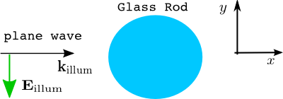
Test example: An incoming plane wave is scattered off an infinite rod.
In this section we use fixed project parameters: The surroundings consists of air. The incoming light field has a vacuum wavelength of  and is polarized in
  -direction with amplitude equal to one. Hence, the illuminating field is given as
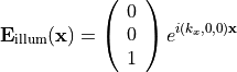
with  . The glass rod has a cross-section diameter of
  and a refractive index of
  , which gives a relative permittivity of
 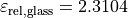 .
.
The input files to this project are given below. The project file mie2D.jcmp defines two post-processes. The first post-process computes the electromagnetic energy flux of the scattered field into the exterior domain. Up to normalization this is the integral scattering cross-section. The second post-process exports the computed field onto a Cartesian mesh.
The following driver run.py shows how to run the project in Python:
1 2 3 4 5 6 7 8 9 10 11 12 13 14 15 16 17 18 19 20 21 22 23 24 25 26 27 28 29 | import jcmwave
# run the project
results = jcmwave.solve('mie2D.jcmp')
# get scattering cross section
scattering_cross_section = results[1]['ElectromagneticFieldEnergyFlux'][0][0]
print ('\nscattering cross section: %.8g\n' % scattering_cross_section.real )
# plot exported cartesian grid within python
cfb = results[2]
amplitude = cfb['field'][0]
intensity = (amplitude.conj()*amplitude).sum(2).real
from matplotlib.pyplot import *
pcolormesh(cfb['X'], cfb['Y'], intensity, shading='gouraud')
axis('tight')
gca().set_aspect('equal')
gca().xaxis.major.formatter.set_powerlimits((-1, 0))
gca().yaxis.major.formatter.set_powerlimits((-1, 0))
show()
|
Line 1 imports the JCMsuite interface module jcmwave.
In line 5, the project is solved.
The computed data is returned as a list, where results[0] refers to the fieldbag and the subsequent entries refer to result data of the post-processes.
This way one can extract the scattering cross-section in line 8.
In lines 12-14 we compute the intensity on a regular Cartesian grid to which the field has been exported.
Using Matplotlib the intensity is plotted (lines 16-21), see Figure “Intensity. Pseudo-color intensity plot as produced by the driver run.py.”.
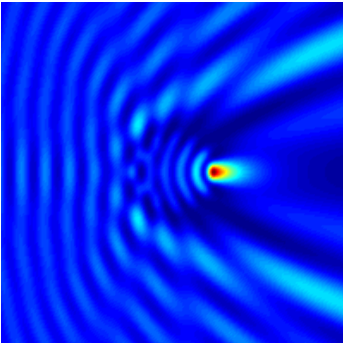
Intensity. Pseudo-color intensity plot as produced by the driver run.py.
For visualization of the computed fields you may also use the JCMview-tool which is available within Python by the wrapper view.py:
jcmwave.view(results[0]['file'])
Here, results[0]['file'] is the file path to the computed solution fieldbag.
In the above driver run.py we have used the command solve, which automatically created the finite element mesh, solved the problem and loaded the result data. Often, when setting up a new project, you may first want to check if the geometry has been defined properly. To do this, call the mesh generator separately (driver run_geo.py):
import jcmwave

# generate mesh file only
jcmwave.geo('.')

# open grid.jcm in JCMview
jcmwave.view('grid.jcm')
The next section Keyword Substitution shows how the test problem is parameterized.
.jcm Input Files
layout.jcm [ASCII]
 1
 2
 3
 4
 5
 6
 7
 8
 9
10
11
12
13
14
15
16
17
18
19
20
21
22
23
24
25
26
27
28
29
Layout {
  UnitOfLength = 1e-6

  MeshOptions {
    MaximumSidelength = 0.1
  }

  # Computational domain
  Parallelogram {
    DomainId = 1
    Width = 4
    Height = 4

    # set transparent boundary conditions
    BoundarySegment {
      BoundaryClass = Transparent
    }
  }

  # Scatterer (rod)
  Circle {
    DomainId = 2
    Radius = 0.5
    RefineAll = 4
  }
}
materials.jcm [ASCII]
 1
 2
 3
 4
 5
 6
 7
 8
 9
10
11
12
13
14
15
# material properties for the surroundings (air)
Material {
  DomainId = 1
  RelPermittivity = 1.0
  RelPermeability = 1.0
}

# material properties the glass rod
Material {
  DomainId = 2
  RelPermittivity = 2.3104 # 1.52^2
  RelPermeability = 1.0
}
sources.jcm [ASCII]
 1
 2
 3
 4
 5
 6
 7
 8
 9
10
SourceBag {
  Source {
    ElectricFieldStrength {
      PlaneWave {
        K = [1.14239732857811e7 0.0 0.0]
        Amplitude = [0 0 1]
      }
    }
  }
}
mie2D.jcmp [ASCII]
 1
 2
 3
 4
 5
 6
 7
 8
 9
10
11
12
13
14
15
16
17
18
19
20
21
22
23
24
25
26
27
28
29
30
31
32
33
34
35
36
37
38
39
40
41
Project {
  InfoLevel = 3
  Electromagnetics {
    TimeHarmonic {
      Scattering {
        FieldComponents = Electric
        Accuracy {
					FiniteElementDegree = 3
          Refinement {
            MaxNumberSteps = 0
            PreRefinements = 0
          }
        }
      }
    }
  }
}

# computes the energy flux of the scattered field into the exterior domain
PostProcess {
  FluxIntegration {
    FieldBagPath = "./mie2D_results/fieldbag.jcm"
    OutputFileName = "./mie2D_results/energyflux_scattered.jcm"
    OutputQuantity = ElectromagneticFieldEnergyFlux
    InterfaceType = ExteriorDomain
  }
}

# exports computed field on cartesian grid
PostProcess {
  ExportFields {
    FieldBagPath = "./mie2D_results/fieldbag.jcm"
    OutputFileName = "./mie2D_results/fieldbag_cartesian.jcm"
    Cartesian {
      NGridPointsX=200
      NGridPointsY=200
    }
  }
}