Quarter-Wave Plate
The chiral response of optical scatterers may be computed in JCMsuite using the formalism of the optical chirality and
the built-in Chiral Quantities. It has been shown that the time-harmonic optical chirality density obeys a local
continuity equation [1]. This enables the analysis of chiral behaviour analogous to the study of electromagnetic energy.
Circularly polarized plane waves are eigenstates of the optical chirality. Accordingly, the near-field optical chirality density is closely connected to circular polarization. Quarter-wave plates converting linear into circular polarization are well-known in geometric optics. They are made of birefringent, e.g. anisotropic, materials. The thickness of the wave plate is a quarter of the difference of the wavelength of the ordinary (x-) and the extraordinary (z-) polarization. The incident plane wave is linearly polarized in xz-direction and propagates in -y-direction as depicted in the figure below.

Conservation of energy and optical chirality for a quarter-wave plate
Due to the linear polarization, the incident chirality flux vanishes  . For a perfect quarter-wave plate, the reflected flux
  would vanish and the transmitted chirality flux
  in units of a circularly polarized plane wave. From geometric optics, we expect the change of polarization or the conversion of chirality takes place in the volume (
 ) of the wave plate due to its anisotropy. For the rigorous solution of Maxwell’s equations, slight deviations from this simplified model occur.
In the near-field, chirality conversion takes place due to both anisotropy and variations in the material parameters [1].
The volumetric contribution can be computed within JCMsuite with the DensityIntegration of the AnisotropicElectricChirality yielding  . The conversion is analogous to the energy absorption
  .
For the piecewise constant materials of this example, chirality conversion at the interfaces is computed by the FluxIntegration of the ElectromagneticChiralityConversionFlux. Its real part yields
.
For the piecewise constant materials of this example, chirality conversion at the interfaces is computed by the FluxIntegration of the ElectromagneticChiralityConversionFlux. Its real part yields  .
.
Finally, the reflected () and transmitted ( ) optical chirality fluxes are given by the real parts of the FluxIntegration of the ElectromagneticChiralityFlux with the InterfaceType
 ExteriorDomain.
Due to the conservation of optical chirality, it holds

for arbitrary materials and electromagnetic fields. This is similar to the conservation of energy, which reads as  .
.
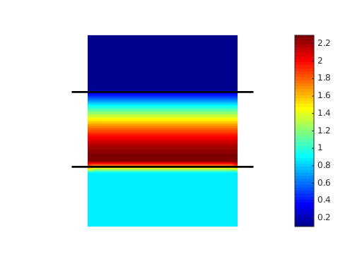
The optical chirality density  is shown below.
 |
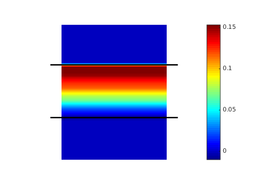 |
This is obtained from the OutputQuantity MagneticChiralityDensity and AnisotropicElectricChiralityDensity. Here, the current notation does not distinguish between integrated quantities, e.g. or  , and densities such as
  .
.
Note that the anisotropic chirality densities are computationally more expensive than their isotropic counter parts. Since the involved materials are non-magnetic ( ), it is sufficient to compute the (isotropic) magnetic chirality density. Note also that the anisotropic quantities are only accessible for the solution with the respective
 FieldComponents Electric or Magnetic. This is due to an additionally required derivative of the fields.
The analysis of the near-field of the quarter-wave plate (see figure above) confirms the expectations from geometric optics: the change of polarization takes place in the volume (and at the interfaces) of the wave-plate and is zero in the surrounding air. The optical chirality density of the downward propagating (output) plane wave is nearly unity in units of the chirality density of a circularly plane wave. It is found that the output polarization is almost completely circularly polarized since  .
Higher performance of the device such as lower reflection could be obtained by optimizing its thickness.
.
Higher performance of the device such as lower reflection could be obtained by optimizing its thickness.
Bibliography
| [1] | (1, 2) Philipp Gutsche, Lisa V. Poulikakos, Martin Hammerschmidt, Sven Burger, and Frank Schmidt. Time-harmonic optical chirality in inhomogeneous space. In SPIE OPTO, Vol.9756, pages 97560X. International Society for Optics and Photonics, 2016. |