How to choose the right optimization method?
At JCMwave we perform optimizations of photonic devices such as light sources, metamaterials, or solar cells on a regular basis using JCMsuite's analysis and optimization toolkit. In this blog post we want to share some insights in common optimization methods and the question which method is the best for which problem. We focus on problems of shape optimization with a moderate number of parameters ranging from 1 to say 100. That is, many methods designed for problems with a very large number of parameters (such as topology optimization or optimization of neural networks) are not considered. Moreover, we assume that the objective function is sufficiently smooth (at least one time differentiable) and can be observed without noise. This is the usual case for the simulation-based shape optimization of physical systems.
Without loss of generality, we consider minimization problems.
First, we give a short introduction and discussion of several relevant optimization algorithms: L-BFGS-B, downhill simplex, differential evolution, and Bayesian optimization. If you are not interested in the background of these algorithms, you might scroll down to the decision tree on the selection of the best optimization method.
Broyden–Fletcher–Goldfarb–Shanno (BFGS) algorithm
The BFGS algorithm is a second-order method that models the objective function locally by a second-order Taylor expansion. At iteration $k$ at position $\mathbf{x}_k$ it tries to find a step $\mathbf{p}$ to a local minimum of $f$, i.e. $\nabla f(\mathbf{x}_{k}+\mathbf{p})=0$.
Consider the first-order Taylor expansion of the gradient $$\nabla f(\mathbf{x}_k + \mathbf{p}) \approx \nabla f(\mathbf{x}_k) + \mathbf{H}\mathbf{p}, \;\text{where}\; (\mathbf{H})_{i j} = \left.\frac{\partial^2 f}{\partial x_i \partial x_j}\right|_{(\mathbf{x}=\mathbf{x}_k)}. $$ If $f$ is strongly convex $f$ around $\mathbf{x}_{k}$, the Hessian $\mathbf{H}$ is a positive definite matrix that can be inverted. Then, the step evaluates to $$ \mathbf{p} \approx - \mathbf{H}^{-1} \nabla f(\mathbf{x}_k).$$
As long as the objective is not a quadratic function, the step determined by the second-order expansion will not hit a local minimum. Therefore, the algorithm performs a line search in the direction of $\mathbf{p}$ to minimize $f$. That is the next point $\mathbf{x}_{k+1}$ is found by minimizing $f(\mathbf{x}_k + \gamma\mathbf{p})$ over the scalar $\gamma > 0$.
The gradient $\nabla f(\mathbf{x}_k)$ can be approximated by finite differences. However, this is often computationally very expensive. The function $f$ has to be additionally evaluated at small distances $f(\mathbf{x}_k + \delta\mathbf{e}_1),f(\mathbf{x}_k + \delta\mathbf{e}_2),\dots,f(\mathbf{x}_k + \delta\mathbf{e}_d)$. Moreover, a higher precision of the numerical evaluation of $f$ is required to also determine differences of function values with sufficiently high precision. Therefore, the BFGS algorithm should be rather applied, if the derivatives can be determined along with the function value. The FEM solver of JCMsuite, for example, computes derivatives using fast and precise automatic differentiations of all computation steps.
Approximation of the inverse of the Hessian matrix
The exact determination of the Hessian is often numerically too involving. Even when using automatic differentiation, at every computational step $d(d+1)/2$ additional operations have to be performed. Therefore the inverse Hessian $\mathbf{H}^{-1}$ is build up iteratively using the secant equation $$ \nabla f(\mathbf{x}_{k+1}) = \nabla f(\mathbf{x}_{k}) + \mathbf{H}_{k+1}(\mathbf{x}_{k+1}-\mathbf{x}_{k}).$$
The equation doesn't determine $\mathbf{H}_{k+1}^{-1}$ completely. By imposing that the update $\mathbf{H}_{k+1}^{-1}$ of $\mathbf{H}_{k}^{-1}$ leads to a symmetric matrix that fulfills the secant equation and is minimal in the Eucledian norm, i.e. $\min_{\mathbf{H}_{k+1}^{-1}}\left\lVert\mathbf{H}_{k+1}^{-1}-\mathbf{H}_{k}^{-1}\right\rVert$ one obtains the BFGS update rule
$$ \mathbf{H}_{k+1}^{-1} = \left(I - \frac{\mathbf{s} \mathbf{y}^T}{\mathbf{y}^T \mathbf{s}} \right) \mathbf{H}_{k}^{-1} \left(I - \frac{\mathbf{y} \mathbf{s}^T}{\mathbf{y}^T \mathbf{s}} \right) + \frac{\mathbf{s} \mathbf{s}^T}{\mathbf{y}^T \mathbf{s}} $$
with $\mathbf{y} = \nabla f(\mathbf{x}_{k+1}) - \nabla f(\mathbf{x}_{k})$ and $\mathbf{s} = \mathbf{x}_{k+1}-\mathbf{x}_{k}$.
In order to visualize the behavior of the algorithm, we consider two dimensional Himmelblau's function $f(x, y) = (x^2+y-11)^2 + (x+y^2-7)^2$, which has four local minima. The animation below shows that after each line search the search continues into a new direction.
%matplotlib notebook
import scipy.optimize
from utils import OptimizationVisualizer
from IPython.display import HTML, clear_output
ov = OptimizationVisualizer(jac=True)
scipy.optimize.minimize(ov,x0=[0,0],jac=True,method='BFGS')
anim = ov.animate()
clear_output()
HTML(anim.to_jshtml())
L-BFGS-B
In practice one often applies an extension of the BFGS algorithm.
L="limited memory": The full inverse matrix $\mathbf{H}_{k}^{-1}$ does not have to be stored to perform the step computation $\mathbf{p} = - \mathbf{H}_{k}^{-1} \nabla f(\mathbf{x}_k)$. Instead one can use a limited history of previous $\mathbf{y}$ and $\mathbf{s}$ values to iteratively determine $\mathbf{p}$ (see https://en.wikipedia.org/wiki/Limited-memory_BFGS).
B="bound constraints": In order to search within bound or box constraints $l_i \leq x_i \leq u_i$ a set of inactive and active parameters along the gradient direction is first determined and the L-BFGS algorithm is performed on the active parameters.
The restriction of the search space leads to a small improvent of the convergence speed for the Himmelblau's function:
%matplotlib notebook
import scipy.optimize
from utils import OptimizationVisualizer
from IPython.display import HTML, clear_output
ov = OptimizationVisualizer(jac=True)
scipy.optimize.minimize(ov,bounds=[[-6,6],[-6,6]],x0=[0,0],jac=True,method='L-BFGS-B')
anim = ov.animate()
clear_output()
HTML(anim.to_jshtml())
L-BFGS-B converges relatively quickly to a local minimum. To perform a global search for multiple local minima, one can start the algorithm, either sequentially or in parallel, from different initial points. Since the minimizations do not share any information, this approach generally degrades the efficiency. Especially, some of the minimization runs might converge to the same local minimum. Moreover, it is a-priori unclear how many initial points should be chosen for a specific problem.
To sum up, L-BFGS-B has the following advantages and disadvantages:
- Advantages
- Fast convergence to a local minimum
- Scales well for a large number of parameters
- Requires derivatives
- Not as efficient for global optimization.
Downhill simplex algorithm
The downhill simplex algorithm, also known as Nelder-Mead algorithm after its inventors, does not require derivative information. It performs a local minimization by repeating the following operations:
Start An $d$ dimensional simplex $\mathbf x_1, \ldots, \mathbf x_{d+1}$.
1. Order according to the values at the vertices: $f(\mathbf x_1) \leq f(\mathbf x_2) \leq \cdots \leq f(\mathbf x_{d+1})$ and calculate the centroid $\mathbf x_o$ of $\mathbf x_{1},\cdots,\mathbf x_{d}$.
2. Reflection Compute reflected point $\mathbf x_r = \mathbf x_o + (\mathbf x_o - \mathbf x_{n+1})$. If $f(\mathbf x_1) \leq f(\mathbf x_r) < f(\mathbf x_d)$, replace the worst point $\mathbf x_{d+1}$ with $\mathbf x_r$, and go to step 1.
3. Expansion If $f(\mathbf x_r) < f(\mathbf x_1)$, then compute the expanded point $\mathbf x_e = \mathbf x_o + 2 (\mathbf x_r - \mathbf x_o)$. If $f(\mathbf x_e) < f(\mathbf x_r)$, replace the worst point $\mathbf x_{d+1}$ with $\mathbf x_e$ and go to step 1; else replace the worst point $\mathbf x_{d+1}$ with $\mathbf x_r$ and go to step 1.
4. Contraction If $f(\mathbf x_r) \geq f(\mathbf x_d)$, compute contracted point $\mathbf x_c = \mathbf x_o + 0.5(\mathbf x_{d+1} - \mathbf x_o)$. If $f(\mathbf x_c) < f(\mathbf x_{d+1})$, replace the worst point $\mathbf x_{d+1}$ with $\mathbf x_c$ and go to step 1.
5. Shrink Replace all points except the best ($\mathbf x_1$) with $\mathbf x_i = \mathbf x_1 + 0.5(\mathbf x_i - \mathbf x_1)$ and go to step 1.
In the following animation, the current simplex is shown as a triangle, and the trial points (reflection, expansion, or contraction) are shown as additional points:
%matplotlib notebook
import scipy.optimize
from utils import OptimizationVisualizer
from IPython.display import HTML, clear_output
ov = OptimizationVisualizer(jac=False)
scipy.optimize.minimize(ov,x0=[0,0],method='Nelder-Mead',options=dict(
initial_simplex=[[-0.5,0],[0,-0.75],[0.5,0]]))
anim = ov.animate(show_simplex=True)
clear_output()
HTML(anim.to_jshtml())
Clearly, downhill simplex requires more function evaluations to get, say, a value below $1.0$ ($16$ evaluations) in comparison to L-BFGS-B ($9$ evaluations). However, if no derivative information is available, it is typically more efficient. In order to determine all partial derivatives at each iteration by finite differences, L-BFGS-B would require $3\cdot9=27$ evaluations. As in the case of L-BFGS-B one can use the downhill-simplex method also for globalized optimizations using a multi-start approach.
Altogether, the downhill-simplex method has the following advantages and disadvantages:
- Advantages
- Fast convergence to a local minimum
- No derivatives required
- Slower convergence than L-BFGS-B
- Not as efficient for global optimization
Differential Evolution
Differential evolution is a heuristic optimization approach that searches globally for a minimum of the function. It belongs to the family of evolutionary algorithms. The algorithm is initialized with a random or pseudo-random population of $M$ agents. It comes in many flavors. However, one of the most common procedures is to update the population according to the following steps:
- Pick randomly three other agents $a,b,c$
- Pick randomly some dimensions $I=\{i_1,i_2,\cdots\}$ according to a crossover probability $CR$
- $x'=x,\; x_i'=a_i+F(b_i-c_i)\; \forall i \in I$ with differential weight $F$
- Replace $x$ by $x'$ in the population if $x'$ is fitter
The following animation shows the behavior of differential evolution. If you download the jupyter notebook and run the cell below multiple times, you will see that differential evolution can converge to any of the four minima.
%matplotlib notebook
import scipy.optimize
from utils import OptimizationVisualizer
from IPython.display import HTML, clear_output
ov = OptimizationVisualizer(jac=False)
scipy.optimize.differential_evolution(ov,bounds=[[-6,6],[-6,6]],popsize=5,maxiter=10)
anim = ov.animate(population_size=5*2)
clear_output()
HTML(anim.to_jshtml())
Differential evolution requires much more function evaluations in order to probe the parameter space globally before it converges to one of the local minima. On the other hand it is not easily trapped in a local minimum with bad performance.
Altogether, the differential evolution has the following advantages and disadvantages:
- Advantages
- Probes the parameter space globally
- No derivatives required
- Slower convergence than L-BFGS-B and downhill simplex
Other evolutionary algorithms are for example particle swarm optimization and CMA-ES. While they can perform very differently for a specific optimization problem, they share roughly the same advantages and disadvantages compared to other optimization methods.
Bayesian optimization
Bayesian optimization is very different from all above methods. It is a model-based optimization method that builds up a stochastic model of the objective function $f$ based on all previous function evaluations. This contrasts the other approaches that have only limited information of the optimization history. Take for example the downhill simplex method: It memorizes only the position and function values of the $d+1$ points included in the current simplex. Evolutionary methods store more information, but that don't use most of it. For example, the movement of particle in particle swarm optimization is independent of the positions of all the other particles. Most frequently, the stochastic model is built up using Gaussian process regression (GPR). GPR performs a Bayesian inference in order to predict the most probable function value and its uncertainty. Hence, it uses all information in a stochastically (almost) optimal way. It can also include derivative information into the Bayesian inference, if they are available.
The mathematical background of Gaussian process regression has been introduced in a previous blog post. A further blog post was dedicated to the rationale behind Bayesian optimization.
The following animation underlines the fundamental difference of Bayesian optimization. While all other methods were converging (i.e. getting stuck) to one of the local minima, Bayesian optimization is in fact probing all minima. If one of the minima would be slightly better than the others, only Bayesian optimization would find this minimum with certainty.
%matplotlib notebook
import scipy.optimize
from time import sleep
from utils import OptimizationVisualizer
from IPython.display import HTML, clear_output
ov = OptimizationVisualizer(jac=True)
import numpy as np
import os,sys
#This requires JCMsuite to be installed.
sys.path.append(os.path.join(os.getenv('JCMROOT'), 'ThirdPartySupport', 'Python'))
import jcmwave
# Definition of the search domain
domain = [
{'name': 'x1', 'type': 'continuous', 'domain': (-6,6)},
{'name': 'x2', 'type': 'continuous', 'domain': (-6,6)}
]
# Creation of the optimization study object. This will automatically
# open a browser window with a dashboard showing the optimization progress.
client=jcmwave.optimizer.client(port=4554)
study = client.create_study(domain=domain, name="Example")
study.set_parameters(max_iter=50)
# Definition of the objective function that will be minimized
def objective(x1,x2):
sleep(3)
val,jac = ov(np.array([x1,x2]))
observation = study.new_observation()
observation.add(val)
observation.add(derivative='x1', value=jac[0])
observation.add(derivative='x2', value=jac[1])
return observation
# set the objective function and run the optimziation loop
study.set_objective(objective)
study.run()
anim = ov.animate()
clear_output()
HTML(anim.to_jshtml())
For simulation-based optimization, Bayesian optimization is often an order of magnitude faster than the other optimization methods (see e.g. this blog post). So why not always use Bayesian optimization? From our experience there can be two reasons to do this:
- Learning and evaluating the stochastic model requires an increasing amount of time. If the evaluation of the objective function takes only a few seconds, it might be more time efficient to use a different method.
- You have very good starting parameter values on you want to converge to the local minimum in a few steps. Note that gradient-based Bayesian optimization can be also used as a local optimization and can outperform L-BFGS-B for a moderate number of parameters (see here or here)
Due to the predictive power of the underlying stochastic model, Bayesian optimization has many advantages:
- Advantages
- Runs a truly global minimization, i.e. it does not get stuck in local minima
- No derivatives required, but they can be used to speed up the optimization
- Extensions of Bayesian optimization allow for optimization of noisy functions, for mixed continuous and discrete parameter spaces, for parallel evaluations of the objective, for non-linear constraints, for local optimizations, and for much more.
- Bayesian optimization has a significant computational overhead and should be only used for expensive objective functions.
Conclusion
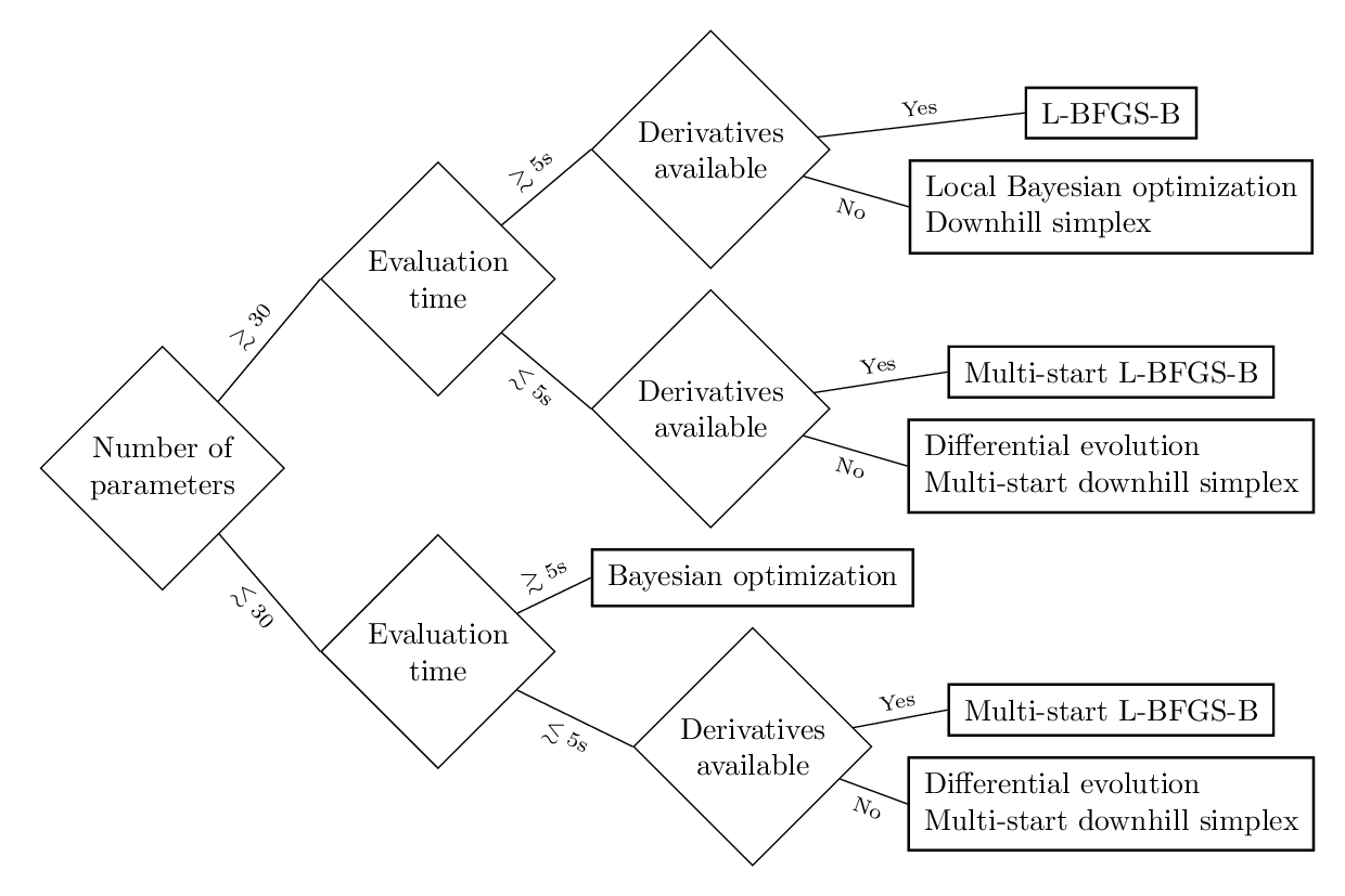
The following decision tree sums up all the advantages and disadvantages of the described optimization methods. The decision is based on the number of free parameters, the evaluation time of the objective function and the availability of derivatives. Of course, the thresholds (30 free parameters and 5 seconds evaluation time) are not strict but are only meant to provide a feeling for the corresponding orders of magnitude.
If you have any question regarding the right choice of the optimization method and its settings in JCMsuite's analysis and optimization toolkit, feel free to write us an email to info@jcmwave.com.
Additional Resources
- Download a free trial version of JCMsuite.
- Tutorial example on Bayesian optimization based on Gaussian process regression.
- Documentation of JCMsuite's Analysis and Optimization Toolkit for Python and Matlab.
- Publication on benchmark of Bayesian optimization against other optimization methods: Schneider, P. I., Garcia Santiago, X., Soltwisch, V., Hammerschmidt, M., Burger, S., & Rockstuhl, C. (2019). Benchmarking five global optimization approaches for nano-optical shape optimization and parameter reconstruction. ACS Photonics, 6(11), 2726-2733. (arXiv link)